1. Linear Systems and Matrices

Linear Equations and Systems

A linear equation in variables $x_1, \ldots, x_n$ has the form

$$a_1x_1 + a_2x_2 + \cdots + a_nx_n = b,$$

where the coefficients $a_i$ and constant $b$ are real numbers. Variables appear only to the first power: terms such as $x^2$, $x_1x_2$, or $\sqrt{x_1}$ are not linear.

A linear system is a collection of linear equations in the same variables. A solution is an assignment of values to every variable that satisfies every equation simultaneously. The solution set contains all such assignments.

Two systems are equivalent when they have the same solution set.

Geometry in Two Variables

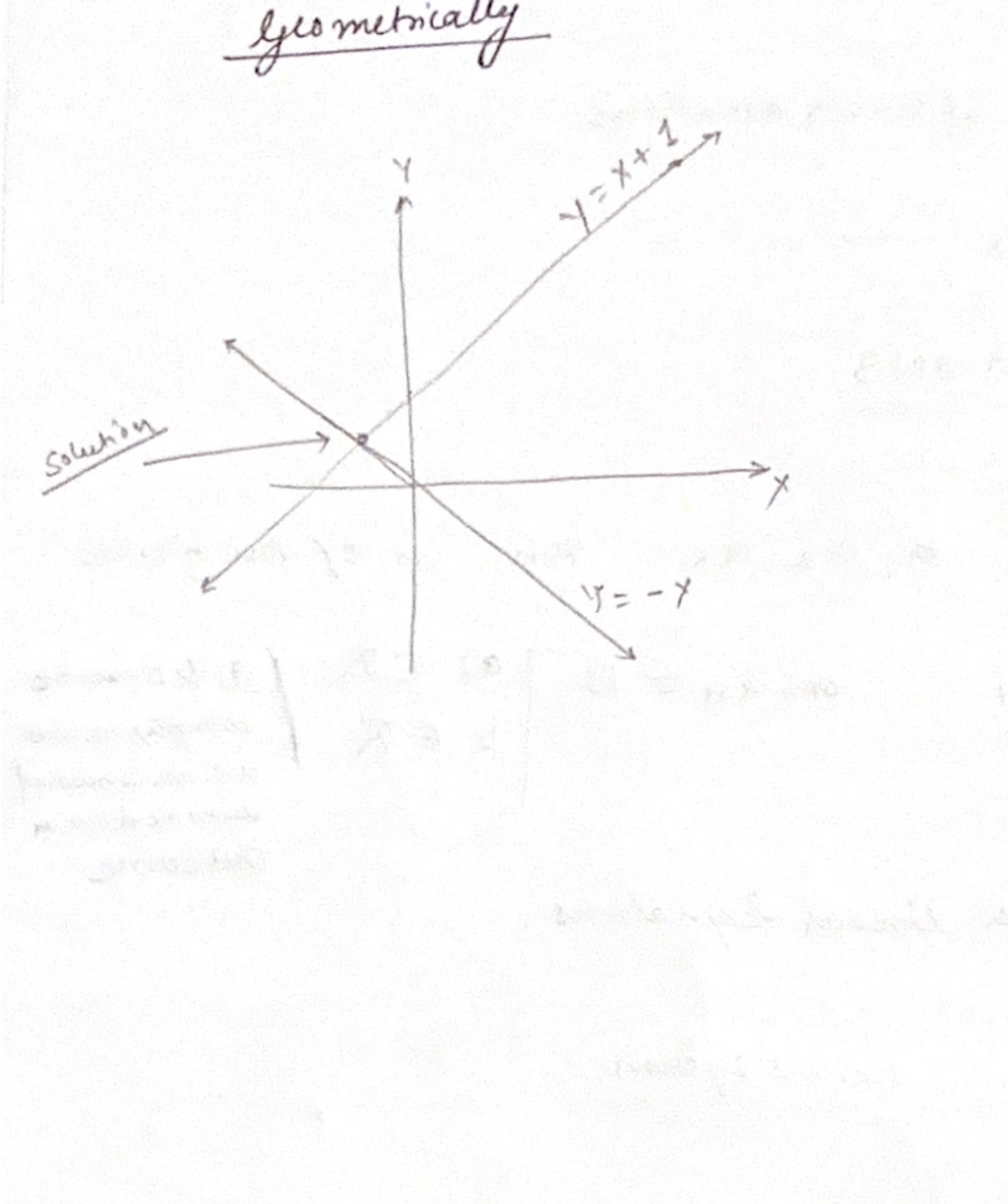
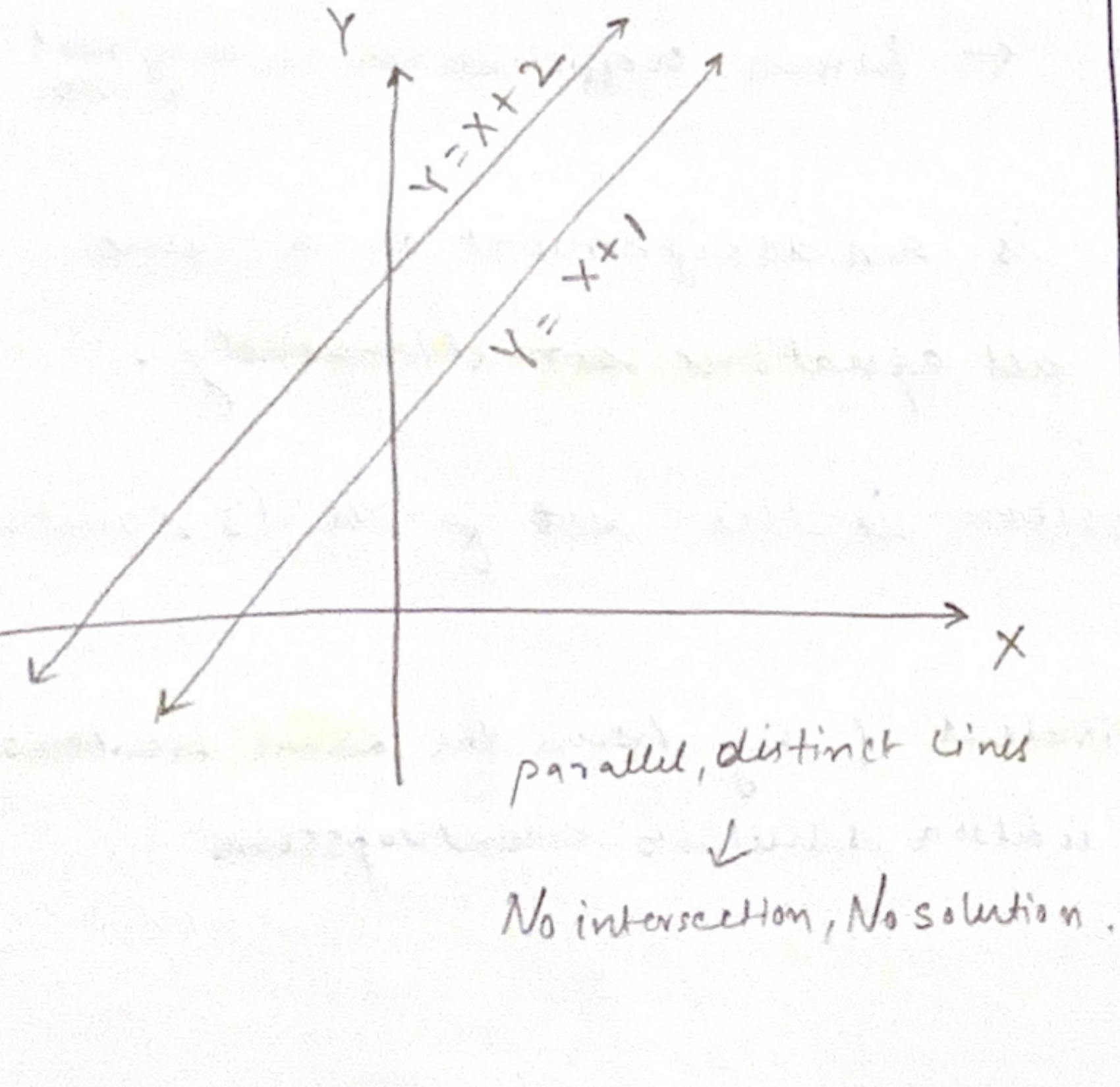
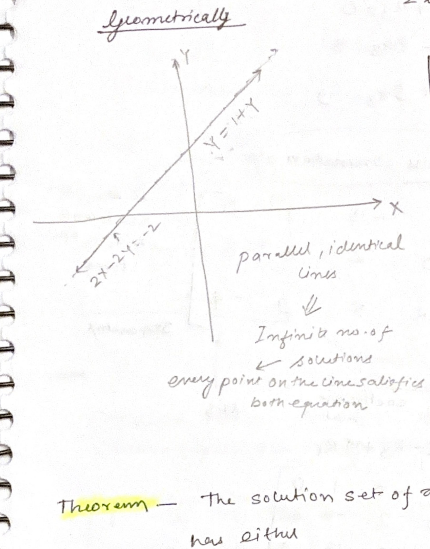
Each linear equation in two variables represents a line. A system's solutions are the points common to all its lines:

Geometry	Number of solutions
Lines intersect once	One solution
Distinct parallel lines	No solution
Same line	Infinitely many solutions

In higher dimensions, equations represent planes or hyperplanes, and solutions lie in their intersection.

Examples

1. Unique solution

   $$\begin{aligned} -x + y &= 1 \\ x + y &= 0 \end{aligned} \quad\Longrightarrow\quad (x,y)=\left(-\frac12,\frac12\right).$$

2. No solution

   $$-x+y=1,\qquad -x+y=2$$

   The equations require the same expression to equal two different values.

   

3. Infinitely many solutions

   $$-x+y=1,\qquad 2x-2y=-2$$

   The second equation is $-2$ times the first. The systems are equivalent, and their solution set is

   $$(x,y)=(t,t+1),\qquad t\in\mathbb R.$$

Theorem - a solution set of any linear system has either

• no solutions
• a unique solution
• infinitely many solutions.

A system of equations is called consistent if it has one or many solutions. If it has no solutions, it is called inconsistent.

Matrix Form

A system of $m$ equations in $n$ variables can be written as

$$A\mathbf{x}=\mathbf{b},$$

where $A\in\mathbb R^{m\times n}$ is the coefficient matrix, $\mathbf{x}\in\mathbb R^n$ is the unknown vector, and $\mathbf{b}\in\mathbb R^m$ is the right-hand-side vector.

The augmented matrix $[A\mid\mathbf b]$ appends the right-hand side as a final column. For example,

$$\begin{aligned} x_1-2x_2+x_3 &= 0 \\ 2x_2-8x_3 &= 8 \\ -4x_1+5x_2+9x_3 &= -9 \end{aligned} \quad\longleftrightarrow\quad \left[\begin{array}{rrr|r} 1 & -2 & 1 & 0 \\ 0 & 2 & -8 & 8 \\ -4 & 5 & 9 & -9 \end{array}\right].$$

Gaussian Elimination

Gaussian elimination applies elementary row operations to an augmented matrix. Each operation produces an equivalent system and preserves its solution set.

1. Swap two rows: $R_i\leftrightarrow R_j$.
2. Multiply a row by a nonzero scalar: $R_i\leftarrow cR_i$, $c\ne0$.
3. Add a multiple of one row to another: $R_i\leftarrow R_i+cR_j$.

Elementary Matrices

An elementary matrix is obtained by applying one elementary row operation to the identity matrix $I_n$. Left multiplication by this matrix applies the same row operation to any $n$-row matrix. For example, applying $R_2\leftarrow R_2+3R_1$ to $I_3$ gives

$$E=\begin{bmatrix}1&0&0\\3&1&0\\0&0&1\end{bmatrix}, \qquad EA=\text{$A$ with row 2 replaced by row 2 plus 3 times row 1}.$$

Row swaps, scaling a row by a nonzero number, and adding a multiple of one row to another each have a corresponding elementary matrix. Every elementary matrix is invertible: its inverse performs the reverse row operation. A sequence of row operations is therefore left multiplication by a product of elementary matrices.

An $n\times n$ matrix $A$ is invertible exactly when it can be written as a product of elementary matrices. If $E_k\cdots E_1A=I_n$, then $A^{-1}=E_k\cdots E_1$.

Continue until the matrix is in row-echelon form, then use back-substitution. Continuing to reduced row-echelon form makes the variables easier to read directly.

Example

The two columns track the same elimination in equation form and matrix form. In each matrix, the last column is the right-hand side.

Normal algebraic elimination	Gaussian elimination with the augmented matrix
Starting system $\begin{aligned}x_1-2x_2+x_3&=0\\2x_2-8x_3&=8\\-4x_1+5x_2+9x_3&=-9\end{aligned}$	Starting augmented matrix $\left[\begin{array}{rrr}1&-2&1\\0&2&-8\\-4&5&9\end{array}\middle\vert\begin{array}{r}0\\8\\-9\end{array}\right]$
Step 1: $(3)\leftarrow(3)+4(1)$ $\begin{aligned}x_1-2x_2+x_3&=0\\2x_2-8x_3&=8\\-3x_2+13x_3&=-9\end{aligned}$	Step 1: $R_3\leftarrow R_3+4R_1$ $\left[\begin{array}{rrr}1&-2&1\\0&2&-8\\0&-3&13\end{array}\middle\vert\begin{array}{r}0\\8\\-9\end{array}\right]$
Step 2: $(3)\leftarrow(3)+\frac32(2)$ $\begin{aligned}x_1-2x_2+x_3&=0\\2x_2-8x_3&=8\\x_3&=3\end{aligned}$	Step 2: $R_3\leftarrow R_3+\frac32R_2$ $\left[\begin{array}{rrr}1&-2&1\\0&2&-8\\0&0&1\end{array}\middle\vert\begin{array}{r}0\\8\\3\end{array}\right]$
Step 3: $(2)\leftarrow(2)+8(3)$ $\begin{aligned}x_1-2x_2+x_3&=0\\2x_2&=32\\x_3&=3\end{aligned}$	Step 3: $R_2\leftarrow R_2+8R_3$ $\left[\begin{array}{rrr}1&-2&1\\0&2&0\\0&0&1\end{array}\middle\vert\begin{array}{r}0\\32\\3\end{array}\right]$
Step 4: $(1)\leftarrow(1)-(3)$ $\begin{aligned}x_1-2x_2&=-3\\2x_2&=32\\x_3&=3\end{aligned}$	Step 4: $R_1\leftarrow R_1-R_3$ $\left[\begin{array}{rrr}1&-2&0\\0&2&0\\0&0&1\end{array}\middle\vert\begin{array}{r}-3\\32\\3\end{array}\right]$
Step 5: $(1)\leftarrow(1)+(2)$ $\begin{aligned}x_1&=29\\2x_2&=32\\x_3&=3\end{aligned}$	Step 5: $R_1\leftarrow R_1+R_2$ $\left[\begin{array}{rrr}1&0&0\\0&2&0\\0&0&1\end{array}\middle\vert\begin{array}{r}0\\32\\3\end{array}\right]$
Step 6: $(2)\leftarrow\frac12(2)$ $\begin{aligned}x_1&=29\\x_2&=16\\x_3&=3\end{aligned}$	Step 6: $R_2\leftarrow\frac12R_2$ RREF $\left[\begin{array}{rrr}1&0&0\\0&1&0\\0&0&1\end{array}\middle\vert\begin{array}{r}29\\16\\3\end{array}\right]$

The RREF directly gives $x_1=29$, $x_2=16$, and $x_3=3$. Thus the unique solution is

$$(x_1,x_2,x_3)=(29,16,3).$$

• Operations do not change the solution set of the Original system of equations. They do change the system of equations, but the changed system also has the same solution set as the original system.
• A row operation can be applied to any matrix, not just one derived from a system of equations. Matrices obtained by applying row operations to another matrix are called row‑equivalent.
• Note that all three row operations are reversible.

Echelon Forms, Pivots, and Variables

The first nonzero entry of a nonzero row is its leading entry, or pivot. The table compares row-echelon form with reduced row-echelon form.

Row-echelon form (REF)	Reduced row-echelon form (RREF)
Conditions - All-zero rows, if any, are below the nonzero rows. - Each row's pivot is to the right of the pivot in the row above it. - Entries below each pivot are zero. - Pivots do not have to equal $1$; entries above a pivot may be nonzero. - A matrix can have more than one REF.	Conditions - The matrix must first satisfy all REF conditions. -Every pivot equals $1$. - Each pivot is the only nonzero entry in its column, so entries both above and below it are zero. - Every matrix has exactly one RREF.
example $\left[\begin{array}{rrr}1&-2&1\\0&2&-8\\0&0&1\end{array}\middle\vert\begin{array}{r}0\\8\\3\end{array}\right]$	example $\left[\begin{array}{rrr}1&0&0\\0&1&0\\0&0&1\end{array}\middle\vert\begin{array}{r}29\\16\\3\end{array}\right]$

The two example matrices are row-equivalent: continuing elimination from the REF on the left produces the RREF on the right. A matrix may be upper triangular without being in REF; REF also requires the pivots to step to the right as you move down the rows.

Every finite matrix can be transformed using elementary row operations into row-echelon form and then into reduced row-echelon form.

• Variables in pivot columns are basic (pivot) variables.
• Variables in non-pivot columns are free variables.

Choose arbitrary values for the free variables, then solve for the basic variables. Writing all variables in terms of parameters gives a parametric form of the solution set.

Consistency and Number of Solutions

A system is consistent if it has at least one solution. Otherwise it is inconsistent.

In an augmented REF or RREF, a row of the form

$$[0\quad 0\quad\cdots\quad 0\mid c],\qquad c\ne0,$$

means $0=c$, so the system is inconsistent. If no such row appears, the system is consistent.

• Inconsistent systems have no solutions.
• A consistent system with no free variables has a unique solution.
• A consistent system with one or more free variables has infinitely many solutions.

Aside

Claim: If a linear system has more variables than equations, a solution always exists.

False. For example, this system has five variables and two equations:

$$\left[\begin{array}{ccccc|c} 1&1&1&1&1&3\\ 0&0&0&0&0&1 \end{array}\right]$$

The second row says $0=1$, so the system is inconsistent and has no solution. Having more variables than equations may give free variables, but it does not guarantee that the system is consistent.

Reading Solutions from RREF

For example,

$$\left[\begin{array}{rrr|r} 1 & 0 & -5 & 1 \\ 0 & 1 & 1 & 4 \\ 0 & 0 & 0 & 0 \end{array}\right]$$

represents $x_1-5x_3=1$ and $x_2+x_3=4$. Let the free variable $x_3=t$. Then

$$\mathbf{x}= \begin{bmatrix}1+5t\\4-t\\t\end{bmatrix} = \begin{bmatrix}1\\4\\0\end{bmatrix} +t\begin{bmatrix}5\\-1\\1\end{bmatrix}, \qquad t\in\mathbb R.$$

By contrast,

$$\left[\begin{array}{rrr|r} 1 & 0 & -\frac43 & 0 \\ 0 & 1 & 0 & 0 \\ 0 & 0 & 0 & 1 \end{array}\right]$$

contains $0=1$ and is inconsistent.

Homogeneous Systems and Null Space

A system is homogeneous when it has the form

$$A\mathbf{x}=\mathbf{0}.$$

It is always consistent because $\mathbf{x}=\mathbf{0}$ is a solution (the trivial solution). A nonzero solution is a non-trivial solution. A homogeneous system has a non-trivial solution exactly when it has at least one free variable.

Why does a free variable allow a non-trivial solution?

If there are no free variables, every variable is a pivot variable, and the homogeneous equations force the only solution to be $\mathbf{x}=\mathbf{0}$. If there is a free variable, assign it a nonzero value; the pivot variables can then be chosen to satisfy the equations, producing a nonzero solution.

For example, in $x+y=0$, let the free variable be $y=1$. Then $x=-1$, so $(-1,1)$ is a non-trivial solution.

The set of solutions to $A\mathbf{x}=\mathbf{0}$ is the null space of $A$, written $\operatorname{N}(A)$. It is a subspace and contains the zero vector.

Homogeneous-System Examples

Example 1: One Free Variable

Consider the homogeneous system in reduced row-echelon form:

$$\left[\begin{array}{rrr|r} 1 & 0 & -\frac43 & 0 \\ 0 & 1 & 0 & 0 \\ 0 & 0 & 0 & 0 \end{array}\right].$$

This represents

$$x_1-\frac43x_3=0,\qquad x_2=0,\qquad 0=0.$$

The pivot variables are $x_1$ and $x_2$, so $x_3$ is free. Set $x_3=t$, where $t\in\mathbb{R}$. Then

$$\mathbf{x}= \begin{bmatrix}\frac43t\\0\\t\end{bmatrix} =t\begin{bmatrix}\frac43\\0\\1\end{bmatrix}, \qquad t\in\mathbb{R}.$$

The solutions are all scalar multiples of one vector, so they form a line through the origin. Every solution vector is mapped to zero by $A$.

Example 2: Two Free Variables

Consider the single homogeneous equation

$$10x_1-3x_2-2x_3=0.$$

Solve for the pivot variable $x_1$:

$$x_1=\frac{3}{10}x_2+\frac15x_3.$$

The variables $x_2$ and $x_3$ are free. Set $x_2=s$ and $x_3=t$, with $s,t\in\mathbb{R}$. Then

$$\mathbf{x}= \begin{bmatrix}\frac{3}{10}s+\frac15t\\s\\t\end{bmatrix} =s\begin{bmatrix}\frac{3}{10}\\1\\0\end{bmatrix} +t\begin{bmatrix}\frac15\\0\\1\end{bmatrix}, \qquad s,t\in\mathbb{R}.$$

The solutions are all linear combinations of two direction vectors, so they form a plane through the origin. Both direction vectors, and every vector in their span, belong to the null space of the coefficient matrix.

The Minus-One Trick

For a homogeneous system in RREF, set one free variable to $-1$ and all other free variables to $0$. The resulting solution gives a null-space basis vector; repeat for each free variable.

For example, consider

$$\begin{bmatrix} 1&3&0&0&3\\ 0&0&1&0&9\\ 0&0&0&1&-4 \end{bmatrix}.$$

Here $x_2$ and $x_5$ are free. Setting $(x_2,x_5)=(-1,0)$ gives $\begin{bmatrix}3&-1&0&0&0\end{bmatrix}^T$; setting $(x_2,x_5)=(0,-1)$ gives $\begin{bmatrix}3&0&9&-4&-1\end{bmatrix}^T$. Thus the general solution is

$$\mathbf{x}=s\begin{bmatrix}3\\-1\\0\\0\\0\end{bmatrix} +t\begin{bmatrix}3\\0\\9\\-4\\-1\end{bmatrix}, \qquad s,t\in\mathbb{R}.$$

Geometry and Parametric Vectors

• A line through the origin can be written $\mathbf{x}=t\mathbf{v}$.
• A plane through the origin can be written $\mathbf{x}=s\mathbf{u}+t\mathbf{v}$.
• Such vector equations describe all linear combinations of the direction vectors.

An expression such as $\mathbf{x}=t\mathbf{v}$ or $\mathbf{x}=s\mathbf{u}+t\mathbf{v}$, with real parameters, is a parametric vector equation. As the parameters vary, it describes the same line or plane as the corresponding equations. When all solutions of a linear system are written as a vector expression with parameters, that expression is the system's parametric vector form.

For example, the earlier RREF solution can be written as

$$\mathbf{x}= \begin{bmatrix}1+5t\\4-t\\t\end{bmatrix} = \begin{bmatrix}1\\4\\0\end{bmatrix} +t\begin{bmatrix}5\\-1\\1\end{bmatrix}, \qquad t\in\mathbb{R}.$$

The first vector is one particular solution; the direction vector is a solution to the corresponding homogeneous system.

More generally, if $A\mathbf{x}=\mathbf{b}$ is consistent, $\mathbf{p}$ is one particular solution, and $\mathbf{v}_1,\ldots,\mathbf{v}_k$ form a basis for the null space of $A$, then every solution has parametric vector form

$$\mathbf{x}=\mathbf{p}+t_1\mathbf{v}_1+\cdots+t_k\mathbf{v}_k, \qquad t_1,\ldots,t_k\in\mathbb{R}.$$

For a homogeneous system, $\mathbf{p}=\mathbf{0}$, so its parametric vector form has no offset and describes a subspace through the origin. A consistent non-homogeneous system's solution set is a translate of the null space; an inconsistent system has no solutions.

Why does this give every solution?

Let $\mathbf{p}$ be one solution, so $A\mathbf{p}=\mathbf{b}$. If $\mathbf{x}$ is any other solution, then

$$A(\mathbf{x}-\mathbf{p})=A\mathbf{x}-A\mathbf{p}=\mathbf{b}-\mathbf{b}=\mathbf{0}.$$

Therefore, the difference $\mathbf{x}-\mathbf{p}$ belongs to the null space of $A$. Conversely, if $\mathbf{z}$ is in that null space, then $A(\mathbf{p}+\mathbf{z})=A\mathbf{p}+A\mathbf{z}=\mathbf{b}+\mathbf{0}=\mathbf{b}$, so adding any null-space vector to $\mathbf{p}$ gives another solution. For a homogeneous system, $\mathbf{b}=\mathbf{0}$ and we can choose $\mathbf{p}=\mathbf{0}$; the solutions are exactly the null-space vectors.

Matrix Operations

Equality of Matrices

Two matrices are equal only if they have the same dimensions and all corresponding entries are equal. For $A,B\in\mathbb{R}^{p\times q}$,

$$A=B\quad\Longleftrightarrow\quad A_{ij}=B_{ij}\text{ for every }1\le i\le p,\ 1\le j\le q.$$

Addition and Scalar Multiplication

Matrices can be added only when they have the same dimensions; add corresponding entries:

$$(A+B)_{ij}=A_{ij}+B_{ij}.$$

For a scalar $c$, scalar multiplication is entrywise: $(cA)_{ij}=cA_{ij}$.

Matrix Multiplication

If $A$ is $p\times q$ and $B$ is $q\times r$, then $AB$ is defined and has size $p\times r$. Its entries are row-by-column dot products:

$$(AB)_{ij}=\sum_{k=1}^{q}A_{ik}B_{kj}.$$

This multiplication rule represents composition of linear transformations. Let $B$ map $\mathbb{R}^r$ to $\mathbb{R}^q$, and let $A$ map $\mathbb{R}^q$ to $\mathbb{R}^p$. Applying $B$ first and then $A$ sends $\mathbf{x}$ to $A(B\mathbf{x})$. Since

$$A(B\mathbf{x})=(AB)\mathbf{x},$$

the single matrix representing the composed transformation is $AB$. Its column $j$ is $A$ applied to column $j$ of $B$, which gives the entry formula above.

Hadamard Product

The Hadamard product (or entrywise product) is defined for matrices $A$ and $B$ with the same dimensions. It multiplies corresponding entries:

$$(A\odot B)_{ij}=A_{ij}B_{ij}.$$

For example,

$$\begin{bmatrix}1&2\\3&4\end{bmatrix} \odot \begin{bmatrix}5&6\\7&8\end{bmatrix} = \begin{bmatrix}5&12\\21&32\end{bmatrix}.$$

Unlike the usual matrix product, it requires identical dimensions and does not use row-by-column dot products.

The inner dimensions must match. Matrix multiplication is generally not commutative: $AB\ne BA$ in general. It is associative and distributive over addition.

Identity and Inverse

The $n\times n$ identity matrix $I_n$ has $1$s on its main diagonal and $0$s elsewhere. It satisfies $AI_n=I_nA=A$ for square $A$.

A square matrix $A$ is invertible if there is a matrix $A^{-1}$ such that

$$AA^{-1}=A^{-1}A=I_n.$$

Not every square matrix is invertible. A non-invertible square matrix is singular. A square matrix is invertible exactly when its RREF is $I_n$ (equivalently, it has a pivot in every column).

To compute an inverse by Gaussian elimination, row-reduce the augmented matrix $[A\mid I_n]$. If the left side reduces to $I_n$, the right side becomes $A^{-1}$:

$$[A\mid I_n]\;\longrightarrow\;[I_n\mid A^{-1}].$$

Why does this give the inverse?

Each column of $I_n$ is a separate right-hand side, a standard basis vector $\mathbf{e}_j$. Row-reducing $[A\mid I_n]$ applies the same operations to all systems $A\mathbf{x}_j=\mathbf{e}_j$ at once. Once the left side is $I_n$, the right-side columns are those solutions; together they form $A^{-1}$ because $AA^{-1}=I_n$.

If the left side cannot be reduced to $I_n$, $A$ is singular and has no inverse. For solving a system $A\mathbf{x}=\mathbf{b}$, elimination is usually preferred to explicitly calculating $A^{-1}$.

Worked 3x3 Example

Find the inverse of

$$A=\begin{bmatrix}0&1&2\\1&0&3\\4&-3&8\end{bmatrix}.$$

Apply each row operation to the entire augmented matrix $[A\mid I_3]$:

$$\left[\begin{array}{ccc|ccc} 0&1&2&1&0&0\\ 1&0&3&0&1&0\\ 4&-3&8&0&0&1 \end{array}\right] \xrightarrow{R_1\leftrightarrow R_2} \left[\begin{array}{ccc|ccc} 1&0&3&0&1&0\\ 0&1&2&1&0&0\\ 4&-3&8&0&0&1 \end{array}\right]$$ $$\xrightarrow{R_3\leftarrow R_3-4R_1} \left[\begin{array}{ccc|ccc} 1&0&3&0&1&0\\ 0&1&2&1&0&0\\ 0&-3&-4&0&-4&1 \end{array}\right] \xrightarrow{R_3\leftarrow R_3+3R_2} \left[\begin{array}{ccc|ccc} 1&0&3&0&1&0\\ 0&1&2&1&0&0\\ 0&0&2&3&-4&1 \end{array}\right]$$ $$\xrightarrow{R_3\leftarrow\frac12R_3} \left[\begin{array}{ccc|ccc} 1&0&3&0&1&0\\ 0&1&2&1&0&0\\ 0&0&1&\frac32&-2&\frac12 \end{array}\right] \xrightarrow{R_1\leftarrow R_1-3R_3} \left[\begin{array}{ccc|ccc} 1&0&0&-\frac92&7&-\frac32\\ 0&1&2&1&0&0\\ 0&0&1&\frac32&-2&\frac12 \end{array}\right]$$ $$\xrightarrow{R_2\leftarrow R_2-2R_3} \left[\begin{array}{ccc|ccc} 1&0&0&-\frac92&7&-\frac32\\ 0&1&0&-2&4&-1\\ 0&0&1&\frac32&-2&\frac12 \end{array}\right] = [I_3\mid A^{-1}].$$

Therefore,

$$A^{-1}=\begin{bmatrix} -\frac92&7&-\frac32\\ -2&4&-1\\ \frac32&-2&\frac12 \end{bmatrix}.$$

Geometric Interpretation of Inverse Matrix

If an invertible matrix $A$ represents a linear transformation, then $A^{-1}$ represents the transformation that undoes it:

$$A^{-1}(A\mathbf{x})=\mathbf{x} \quad\text{and}\quad A(A^{-1}\mathbf{x})=\mathbf{x}.$$

Geometrically, $A$ might rotate, stretch, reflect, or shear every point. Applying $A^{-1}$ reverses those changes and returns each point to its original position. For example, if $A$ doubles lengths, $A^{-1}$ halves them.

A matrix has no inverse if its transformation loses information, such as flattening a plane onto a line: multiple original points then map to the same point, so there's no unique way to undo it.

Inverse and Determinant

This test applies to square matrices. For a square matrix $A$, its determinant tells how its linear transformation scales area or volume:

• If $\det(A)\ne0$, the transformation preserves the full dimension of space. No dimensions collapse, so it is reversible and $A$ has an inverse.
• If $\det(A)=0$, the transformation collapses space into a lower dimension, losing information. It is not reversible, so $A$ has no inverse.

For example,

$$A=\begin{bmatrix}1&2\\2&4\end{bmatrix} \quad\Longrightarrow\quad \det(A)=1\cdot4-2\cdot2=0.$$

Its columns point in the same direction, so the transformation collapses the plane onto a line. Different inputs can produce the same output, preventing an inverse.

Transpose and Useful Properties

The transpose $A^T$ is formed by turning the columns of $A$ into rows: $(A^T)_{ij}=A_{ji}$. A square matrix is symmetric when $A^T=A$; only square matrices can be symmetric.

Transpose and inverse rules

• $(A^T)^T=A$.
• $(cA)^T=cA^T$.
• $(A+B)^T=A^T+B^T$.
• $(AB)^T=B^TA^T$.
• $(A^{-1})^{-1}=A$.
• $(AB)^{-1}=B^{-1}A^{-1}$.
• $(A^T)^{-1}=(A^{-1})^T$.
• $(A+B)^{-1}\ne A^{-1}+B^{-1}$.

Symmetric matrices

• A square matrix is symmetric when $A^T=A$.
• The sum of symmetric matrices is symmetric: if $A^T=A$ and $B^T=B$, then $(A+B)^T=A^T+B^T=A+B$.
• The product of symmetric matrices need not be symmetric. For example, both $A=\begin{bmatrix}1&0\\0&0\end{bmatrix}$ and $B=\begin{bmatrix}0&1\\1&0\end{bmatrix}$ are symmetric, but $AB=\begin{bmatrix}0&1\\0&0\end{bmatrix}$ is not.
• If $A$ is symmetric, then $A^{-1}$ is also symmetric. (given A is invertible)

Vectors

A vector in $\mathbb{R}^m$ is an ordered sequence of $m$ real numbers. For example, $(1,3,-2)$ can be written as a row or column matrix:

$$\begin{bmatrix}1&3&-2\end{bmatrix} \qquad\text{or}\qquad \mathbf{x}=\begin{bmatrix}1\\3\\-2\end{bmatrix}.$$

We typically use column vectors. The transpose turns rows into columns and columns into rows; for example,

$$\begin{bmatrix}1&2&3\\4&5&6\end{bmatrix}^{T} = \begin{bmatrix}1&4\\2&5\\3&6\end{bmatrix}.$$

For a column vector $\mathbf{x}=\begin{bmatrix}1&3&-2\end{bmatrix}^{T}$, the product $\mathbf{x}^{T}\mathbf{x}$ is a $1\times1$ scalar, while $\mathbf{x}\mathbf{x}^{T}$ is a $3\times3$ matrix:

$$\mathbf{x}^{T}\mathbf{x} =\begin{bmatrix}1&3&-2\end{bmatrix} \begin{bmatrix}1\\3\\-2\end{bmatrix} =1^2+3^2+(-2)^2=14, \qquad \mathbf{x}\mathbf{x}^{T} =\begin{bmatrix}1\\3\\-2\end{bmatrix} \begin{bmatrix}1&3&-2\end{bmatrix} =\begin{bmatrix}1&3&-2\\3&9&-6\\-2&-6&4\end{bmatrix}.$$

Geometric Representation

Vectors in $\mathbb{R}^2$ can be drawn as arrows in a plane; vectors in $\mathbb{R}^3$ can be represented as arrows in three-dimensional space. A vector has a direction and a length, but its starting point can be anywhere. Drawing it from the origin is a convention that makes its coordinates easy to read.

Vector addition follows the parallelogram rule. For example, with

$$\mathbf{a}=\begin{bmatrix}2\\1\end{bmatrix}, \qquad \mathbf{b}=\begin{bmatrix}1\\3\end{bmatrix}, \qquad \mathbf{a}+\mathbf{b}=\begin{bmatrix}3\\4\end{bmatrix},$$

place the arrows for $\mathbf{a}$ and $\mathbf{b}$ at the same starting point. Their sum is the diagonal of the parallelogram formed by those arrows.

---

Appendix

1. Linear Regression for Overconstrained Systems

   An overconstrained system has more equations than unknowns. For example,

   $$x=1,\qquad x=3$$

   has no exact solution: no single value of $x$ satisfies both equations. Linear regression handles similar situations by choosing model parameters that minimize the sum of squared errors. For this example, minimize

   $$S(x)=(x-1)^2+(x-3)^2.$$

   The minimum occurs at $x=2$, a compromise between the two observations. It does not satisfy either equation exactly, but it minimizes their combined squared error.

   In linear regression, each equation represents an observation and the unknowns are model parameters. In matrix form, we seek $\mathbf{x}$ such that $A\mathbf{x}$ is close to $\mathbf{b}$. When exact equality is impossible, the usual least-squares objective is

   $$\min_{\mathbf{x}}\|A\mathbf{x}-\mathbf{b}\|_2^2.$$

   More equations than unknowns makes a system overdetermined, but does not by itself guarantee inconsistency. Real-world observations often make the equations inconsistent, for example because of measurement noise.

2. The Inverse of a $2\times2$ Matrix

   For

   $$A=\begin{bmatrix}a&b\\c&d\end{bmatrix},$$

   the determinant is $\det(A)=ad-bc$. If it is nonzero, then

   $$A^{-1}=\frac{1}{ad-bc} \begin{bmatrix} d&-b\\ -c&a \end{bmatrix}.$$

   To remember the formula, swap the diagonal entries, negate the off-diagonal entries, then divide by the determinant. The formula works because

   $$\begin{bmatrix}a&b\\c&d\end{bmatrix} \begin{bmatrix}d&-b\\-c&a\end{bmatrix} = \begin{bmatrix}ad-bc&0\\0&ad-bc\end{bmatrix} =(ad-bc)I_2.$$

   Dividing by $ad-bc$ gives $I_2$. If $ad-bc=0$, the matrix has no inverse.

   For example, if

   $$A=\begin{bmatrix}1&2\\3&4\end{bmatrix},$$

   then $\det(A)=4-6=-2$, so

   $$A^{-1}=-\frac12\begin{bmatrix}4&-2\\-3&1\end{bmatrix} =\begin{bmatrix}-2&1\\\frac32&-\frac12\end{bmatrix}.$$